6. Pandas: Wrangling Operations and Data Visualization

Excel is the most commonly used data analysis software in the world- easy to get a hang off and use

Python with a library like Pandas is a good way to build scale in business analytics. Here are some reasons:

• Ability to work with large data sets is much faster and easier
• Ability to read and work with almost any kind of data.
• Automate repetitive tasks are easier.
• Increase reproducability of work.
• Find and fix errors easier.
• Supports statistics and machine learning capabilities.
• Advanced data visualization capabilities.
• Cross-platform stability — your analysis can be run on any computer.

6.1 Joining Data Frames

pandas provides various facilities for easily combining together Series or DataFrame with various kinds of set logic for the indexes and relational algebra functionality in the case of join / merge-type operations

import pandas as pd
import numpy as np

6.1.1 Merge

• merge()is used to combine two (or more) dataframes on the basis of values of common columns or indexes as in a RDBMS
• If joining columns on columns, the DataFrame indexes will be ignored.
  • Otherwise if joining indexes on indexes or indexes on a column or columns, the index will be passed on

np.random.seed(42)
left = pd.DataFrame({'key': ['a', 'b', 'c', 'd', 'e'], 
                     'dim1':['grp1', 'grp2','grp2','grp3','grp3'],
                     'values': np.random.normal(65,10,5)})
print(left)

  key  dim1     values
0   a  grp1  69.967142
1   b  grp2  63.617357
2   c  grp2  71.476885
3   d  grp3  80.230299
4   e  grp3  62.658466

np.random.seed(42)
right = pd.DataFrame({'key': ['a','b','c','x','y','z'], 
                      'dim2':['aaa', 'aaa','bbb','bbb', 'ccc', 'aaa'],
                      'values': np.random.randint(100, 150, 6)})
print(right)

  key dim2  values
0   a  aaa     138
1   b  aaa     128
2   c  bbb     114
3   x  bbb     142
4   y  ccc     107
5   z  aaa     120

If you want more details on generating data using numpy to generate various types of data please see this tutorial

6.1.1.2 inner join

left

	key	dim1	values
0	a	grp1	69.967142
1	b	grp2	63.617357
2	c	grp2	71.476885
3	d	grp3	80.230299
4	e	grp3	62.658466

right

	key	dim2	values
0	a	aaa	138
1	b	aaa	128
2	c	bbb	114
3	x	bbb	142
4	y	ccc	107
5	z	aaa	120

pd.merge(left,right,how='inner',on='key',)

	key	dim1	values_x	dim2	values_y
0	a	grp1	69.967142	aaa	138
1	b	grp2	63.617357	aaa	128
2	c	grp2	71.476885	bbb	114

pd.merge(left, right, how='inner', right_index=True, left_index=True, suffixes=('_left', '_right'))

	key_left	dim1	values_left	key_right	dim2	values_right
0	a	grp1	69.967142	a	aaa	138
1	b	grp2	63.617357	b	aaa	128
2	c	grp2	71.476885	c	bbb	114
3	d	grp3	80.230299	x	bbb	142
4	e	grp3	62.658466	y	ccc	107

6.1.1.3 left join

pd.merge(left,right,how='left',on='key')

	key	dim1	values_x	dim2	values_y
0	a	grp1	69.967142	aaa	138.0
1	b	grp2	63.617357	aaa	128.0
2	c	grp2	71.476885	bbb	114.0
3	d	grp3	80.230299	NaN	NaN
4	e	grp3	62.658466	NaN	NaN

df= pd.merge(left,right,how='left',on='key')

df.isna().sum()

key         0
dim1        0
values_x    0
dim2        2
values_y    2
dtype: int64

pd.merge(left,right, left_index=True, right_index=True, how='left')

	key_x	dim1	values_x	key_y	dim2	values_y
0	a	grp1	69.967142	a	aaa	138
1	b	grp2	63.617357	b	aaa	128
2	c	grp2	71.476885	c	bbb	114
3	d	grp3	80.230299	x	bbb	142
4	e	grp3	62.658466	y	ccc	107

6.1.1.4 right join

pd.merge(left,right,how='right',on='key')

	key	dim1	values_x	dim2	values_y
0	a	grp1	69.967142	aaa	138
1	b	grp2	63.617357	aaa	128
2	c	grp2	71.476885	bbb	114
3	x	NaN	NaN	bbb	142
4	y	NaN	NaN	ccc	107
5	z	NaN	NaN	aaa	120

6.1.1.5 outer join

pd.merge(left,right,how='outer',on='key')

	key	dim1	values_x	dim2	values_y
0	a	grp1	69.967142	aaa	138.0
1	b	grp2	63.617357	aaa	128.0
2	c	grp2	71.476885	bbb	114.0
3	d	grp3	80.230299	NaN	NaN
4	e	grp3	62.658466	NaN	NaN
5	x	NaN	NaN	bbb	142.0
6	y	NaN	NaN	ccc	107.0
7	z	NaN	NaN	aaa	120.0

pd.merge(left,right, how='outer',left_index=True, right_index=True)

	key_x	dim1	values_x	key_y	dim2	values_y
0	a	grp1	69.967142	a	aaa	138
1	b	grp2	63.617357	b	aaa	128
2	c	grp2	71.476885	c	bbb	114
3	d	grp3	80.230299	x	bbb	142
4	e	grp3	62.658466	y	ccc	107
5	NaN	NaN	NaN	z	aaa	120

6.1.2 Concat

concat() is used to append one (or more) dataframes one below the other (or sideways, depending on whether the axis option is set to 0 or 1

type([1,2])

list

pd.concat([left, right], axis=0)

	key	dim1	values	dim2
0	a	grp1	69.967142	NaN
1	b	grp2	63.617357	NaN
2	c	grp2	71.476885	NaN
3	d	grp3	80.230299	NaN
4	e	grp3	62.658466	NaN
0	a	NaN	138.000000	aaa
1	b	NaN	128.000000	aaa
2	c	NaN	114.000000	bbb
3	x	NaN	142.000000	bbb
4	y	NaN	107.000000	ccc
5	z	NaN	120.000000	aaa

In the above example indexing is not in order.

pd.concat([left, right], axis=0, ignore_index=True)

	key	dim1	values	dim2
0	a	grp1	69.967142	NaN
1	b	grp2	63.617357	NaN
2	c	grp2	71.476885	NaN
3	d	grp3	80.230299	NaN
4	e	grp3	62.658466	NaN
5	a	NaN	138.000000	aaa
6	b	NaN	128.000000	aaa
7	c	NaN	114.000000	bbb
8	x	NaN	142.000000	bbb
9	y	NaN	107.000000	ccc
10	z	NaN	120.000000	aaa

keys: Construct hierarchical index using the passed keys as the outermost level.

df= pd.concat([left, right], axis=0, keys=['left', 'right'])
print(df)

        key  dim1      values dim2
left  0   a  grp1   69.967142  NaN
      1   b  grp2   63.617357  NaN
      2   c  grp2   71.476885  NaN
      3   d  grp3   80.230299  NaN
      4   e  grp3   62.658466  NaN
right 0   a   NaN  138.000000  aaa
      1   b   NaN  128.000000  aaa
      2   c   NaN  114.000000  bbb
      3   x   NaN  142.000000  bbb
      4   y   NaN  107.000000  ccc
      5   z   NaN  120.000000  aaa

s= 'grp2'
left.loc[left.dim1== s]

	key	dim1	values
1	b	grp2	63.617357
2	c	grp2	71.476885

df.loc['left',:]

	key	dim1	values	dim2
0	a	grp1	69.967142	NaN
1	b	grp2	63.617357	NaN
2	c	grp2	71.476885	NaN
3	d	grp3	80.230299	NaN
4	e	grp3	62.658466	NaN

df.loc['right']

	key	dim1	values	dim2
0	a	NaN	138.0	aaa
1	b	NaN	128.0	aaa
2	c	NaN	114.0	bbb
3	x	NaN	142.0	bbb
4	y	NaN	107.0	ccc
5	z	NaN	120.0	aaa

Concatenating column wise

df = pd.concat([left,right],axis=1)
df

	key	dim1	values	key	dim2	values
0	a	grp1	69.967142	a	aaa	138
1	b	grp2	63.617357	b	aaa	128
2	c	grp2	71.476885	c	bbb	114
3	d	grp3	80.230299	x	bbb	142
4	e	grp3	62.658466	y	ccc	107
5	NaN	NaN	NaN	z	aaa	120

pd.concat([left, right], axis=1, join='outer')

	key	dim1	values	key	dim2	values
0	a	grp1	69.967142	a	aaa	138
1	b	grp2	63.617357	b	aaa	128
2	c	grp2	71.476885	c	bbb	114
3	d	grp3	80.230299	x	bbb	142
4	e	grp3	62.658466	y	ccc	107
5	NaN	NaN	NaN	z	aaa	120

My favorite Application of .concat()

# 3 series creatd programmatically 
s1= pd.Series(data=[True,False,True,True,False], index=['a', 'b', 'c', 'd','e'])
s2= pd.Series(data=[100.00,110.00,120.00,130.00,75.00], index=['a', 'b', 'c', 'd','e'])
s3= pd.Series(data=['A','B','C','B','A'], index=['a', 'b', 'c', 'd','e'])
# A list of the 3 series
lst_s= [s1,s2,s3]

# form a dataframe using the series as columns
df= pd.concat(lst_s, axis=1)
df.columns= ['bool_flag', 'dollars', 'category']
df

	bool_flag	dollars	category
a	True	100.0	A
b	False	110.0	B
c	True	120.0	C
d	True	130.0	B
e	False	75.0	A

6.2 Applying functions & aggregation:

• An essential piece of analysis of large data is efficient summarization: computing aggregations like sum(), mean(), median(), min(), and max()
• A measure that gives insight into the nature of a potentially large dataset.

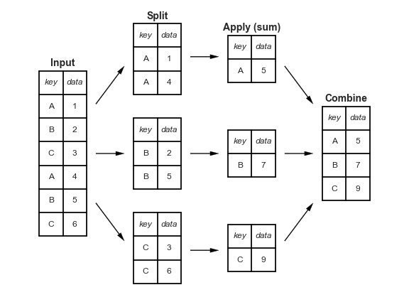
• Simple aggregations can give you a flavor of your dataset, but often we would prefer to aggregate conditionally on some label or index: this is implemented in the so-called groupby operation.

  • The name "group by" comes from a command in the SQL database language

• Split, Apply & Combine: A canonical example of this split-apply-combine operation, where the "apply" is a summation aggregation, is illustrated in this figure:

You may find this interesting

6.2.1 .groupby()

Just to make things a little interesting we shall use Basketball team data!

sport_data = {'Team': ['Nets', 'Nets', 'Clippers', 'Clippers', 'Warriors',
         'Warriors', 'Warriors', 'Warriors', 'Nets', 'Lakers', 'Lakers', 'Nets'],
         'Rank': [1, 2, 2, 3, 3,4 ,1 ,1,2 , 4,1,2],
         'Year': [2014,2015,2014,2015,2014,2015,2016,2017,2016,2014,
                  2015,2017],
         'Points':[876,789,863,673,741,812,756,788,694,701,804,690]}

df=pd.DataFrame(sport_data)
print (df)

        Team  Rank  Year  Points
0       Nets     1  2014     876
1       Nets     2  2015     789
2   Clippers     2  2014     863
3   Clippers     3  2015     673
4   Warriors     3  2014     741
5   Warriors     4  2015     812
6   Warriors     1  2016     756
7   Warriors     1  2017     788
8       Nets     2  2016     694
9     Lakers     4  2014     701
10    Lakers     1  2015     804
11      Nets     2  2017     690

What is the total points won by the basketball teams?

df.groupby(['Team'])['Points'].sum()

Team
Clippers    1536
Lakers      1505
Nets        3049
Warriors    3097
Name: Points, dtype: int64

Output Structure of a .groupby

gf= df.groupby(['Team'])['Points'].sum()
print()
print('What data structure is it? \n', type(gf))
print()
print(' What does the index look like? \n', gf.index)
print()
print('Values:',gf.values)
print()
print('Afer reset_index')
af= gf.reset_index()
print()
print('What data structue now? \n', type(af))
print()
print(' What does the index look like? \n', af.index)
print()
print(' What are the columns? \n', af.columns)

What data structure is it? 
 <class 'pandas.core.series.Series'>

 What does the index look like? 
 Index(['Clippers', 'Lakers', 'Nets', 'Warriors'], dtype='object', name='Team')

Values: [1536 1505 3049 3097]

Afer reset_index

What data structue now? 
 <class 'pandas.core.frame.DataFrame'>

 What does the index look like? 
 RangeIndex(start=0, stop=4, step=1)

 What are the columns? 
 Index(['Team', 'Points'], dtype='object')

af

	Team	Points
0	Clippers	1536
1	Lakers	1505
2	Nets	3049
3	Warriors	3097

We shall us these propeties when we are making graphs

What is the yearly total points by the basketball teams?

df.groupby(['Year', 'Team'])['Points'].sum()

Year  Team    
2014  Clippers    863
      Lakers      701
      Nets        876
      Warriors    741
2015  Clippers    673
      Lakers      804
      Nets        789
      Warriors    812
2016  Nets        694
      Warriors    756
2017  Nets        690
      Warriors    788
Name: Points, dtype: int64

What is the yearly total points by the basketball teams when they were ranked 1?

df.loc[df.Rank==1].groupby(['Year', 'Team'])['Points'].sum()

Year  Team    
2014  Nets        876
2015  Lakers      804
2016  Warriors    756
2017  Warriors    788
Name: Points, dtype: int64

jj=left.merge(right, left_on='key', right_on='key')

jj.loc[jj.dim2=='aaa'].groupby(['dim1','dim2'])['values_x', 'values_y'].sum()

/usr/local/lib/python3.7/dist-packages/ipykernel_launcher.py:1: FutureWarning: Indexing with multiple keys (implicitly converted to a tuple of keys) will be deprecated, use a list instead.
  """Entry point for launching an IPython kernel.

		values_x	values_y
dim1	dim2
grp1	aaa	69.967142	138
grp2	aaa	63.617357	128

6.2.1.1 .agg()

Function to use for aggregating the data. Useful when you have several aggregation functions at the same time passed as a list.

Introduced in Pandas 0.25.0, groupby aggregation with relabelling is supported using “named aggregation” with simple tuples. Python tuples are used to provide the column name on which to work on, along with the function to apply.

df.groupby(['Team'])['Points'].agg([np.min, np.max, np.mean,np.std, np.size])

	amin	amax	mean	std	size
Team
Clippers	673	863	768.00	134.350288	2
Lakers	701	804	752.50	72.831998	2
Nets	690	876	762.25	88.567771	4
Warriors	741	812	774.25	31.899582	4

The list configuration of function is most common. For other implementation data structure look here

Explicitly Labeling Output Columns

df.groupby(['Team']).agg(min_points= ('Points', np.min),max_points= ('Points', np.max), mean_Rank= ('Rank', np.mean))

	min_points	max_points	mean_Rank
Team
Clippers	673	863	2.50
Lakers	701	804	2.50
Nets	690	876	1.75
Warriors	741	812	2.25

6.2.2 .crosstab()

Compute a simple cross-tabulation of two (or more) factors. By default computes a frequency table of the factors unless an array of values and an aggregation function are passed.

pd.crosstab(index=df.Team, columns=df.Year)

Year	2014	2015	2016	2017
Team
Clippers	1	1	0	0
Lakers	1	1	0	0
Nets	1	1	1	1
Warriors	1	1	1	1

pd.crosstab(index=df['Team'], columns=df['Year'], values=df['Points'], aggfunc='sum')

Year	2014	2015	2016	2017
Team
Clippers	863.0	673.0	NaN	NaN
Lakers	701.0	804.0	NaN	NaN
Nets	876.0	789.0	694.0	690.0
Warriors	741.0	812.0	756.0	788.0

6.2.3 .pivot()

• Return reshaped DataFrame organized by given index / column values.

Reshape data (produce a “pivot” table) based on column values. Uses unique values from specified index / columns to form axes of the resulting DataFrame. This function does not support data aggregation, multiple values will result in a MultiIndex in the columns.

df.pivot(index='Team', columns='Year', values='Points')

Year	2014	2015	2016	2017
Team
Clippers	863.0	673.0	NaN	NaN
Lakers	701.0	804.0	NaN	NaN
Nets	876.0	789.0	694.0	690.0
Warriors	741.0	812.0	756.0	788.0

df.groupby(['Year', 'Team'])['Points'].sum().reset_index().pivot(index='Team', columns='Year', values='Points')

Year	2014	2015	2016	2017
Team
Clippers	863.0	673.0	NaN	NaN
Lakers	701.0	804.0	NaN	NaN
Nets	876.0	789.0	694.0	690.0
Warriors	741.0	812.0	756.0	788.0

6.3 Pandas .apply()

-'apply' function along a axis, instad of looping through it.

• While working with tabular data, you must specify an axis you want your function to act on (0 for columns; and 1 for rows).
• You can apply a defined function or a use the lambda function to iterate over the rows of the dataframe

df

	Team	Rank	Year	Points
0	Nets	1	2014	876
1	Nets	2	2015	789
2	Clippers	2	2014	863
3	Clippers	3	2015	673
4	Warriors	3	2014	741
5	Warriors	4	2015	812
6	Warriors	1	2016	756
7	Warriors	1	2017	788
8	Nets	2	2016	694
9	Lakers	4	2014	701
10	Lakers	1	2015	804
11	Nets	2	2017	690

6.3.1 Pandas .apply() on single column

def f(x):
  if x >= 806:
    return('High')
  else:
    return('Low')

f(900)

'High'

df['Scr_flg']= df.Points.apply(lambda x: f(x))

df

	Team	Rank	Year	Points	Scr_flg
0	Nets	1	2014	876	High
1	Nets	2	2015	789	Low
2	Clippers	2	2014	863	High
3	Clippers	3	2015	673	Low
4	Warriors	3	2014	741	Low
5	Warriors	4	2015	812	High
6	Warriors	1	2016	756	Low
7	Warriors	1	2017	788	Low
8	Nets	2	2016	694	Low
9	Lakers	4	2014	701	Low
10	Lakers	1	2015	804	Low
11	Nets	2	2017	690	Low

6.3.2 Pandas .apply() on > 1 column

def g(x,y):
  if (x==1) & (y=='High'):
    return('11')
  elif (x!=1) & (y=='High'):
    return('01')
  else:
    return('00')

Watchout!! The above function is built to be good for single variables and scalars

g(4, 'Low')

'00'

df['rank_score_flg']=df.apply(lambda x: g(x['Rank'], x['Scr_flg']), axis=1)

df

	Team	Rank	Year	Points	Scr_flg	rank_score_flg
0	Nets	1	2014	876	High	11
1	Nets	2	2015	789	Low	00
2	Clippers	2	2014	863	High	01
3	Clippers	3	2015	673	Low	00
4	Warriors	3	2014	741	Low	00
5	Warriors	4	2015	812	High	01
6	Warriors	1	2016	756	Low	00
7	Warriors	1	2017	788	Low	00
8	Nets	2	2016	694	Low	00
9	Lakers	4	2014	701	Low	00
10	Lakers	1	2015	804	Low	00
11	Nets	2	2017	690	Low	00

6.4 Statistical Functions in pandas

List of available function that typically finds use

1. count() Number of non-null observations
2. sum() Sum of values
3. mean() Mean of Values [average]
4. median() Median of Values [cenral value]
5. mode() Mode of values [most common value]
6. std() Standard Deviation of the Values [spread of data]
7. min() Minimum Value [lowest value]
8. max() Maximum Value [Highest value]
9. abs() Absolute Value [non-negaive number component]
10. prod() Product of Values
11. cumsum() Cumulative Sum [running sum by dimension]
12. cumprod() Cumulative Product [product and sum]

Note: − Since DataFrame is a Heterogeneous data structure. Generic operations don’t work with all functions.

df.sum()

Team              NetsNetsClippersClippersWarriorsWarriorsWarrio...
Rank                                                             26
Year                                                          24182
Points                                                         9187
Scr_flg                     HighLowHighLowLowHighLowLowLowLowLowLow
rank_score_flg                             110001000001000000000000
dtype: object

df.median( axis=0)

Rank                 2.0
Year              2015.0
Points             772.0
rank_score_flg       0.0
dtype: float64

df.groupby('Team')['Points'].agg('mean')

Team
Clippers    768.00
Lakers      752.50
Nets        762.25
Warriors    774.25
Name: Points, dtype: float64

df.groupby('Team')['Points'].agg('describe')

	count	mean	std	min	25%	50%	75%	max
Team
Clippers	2.0	768.00	134.350288	673.0	720.50	768.0	815.50	863.0
Lakers	2.0	752.50	72.831998	701.0	726.75	752.5	778.25	804.0
Nets	4.0	762.25	88.567771	690.0	693.00	741.5	810.75	876.0
Warriors	4.0	774.25	31.899582	741.0	752.25	772.0	794.00	812.0

6.5 Plots & Graphs in pandas

matplotlib is a Python package used for data plotting and visualisation. It is a useful complement to pandas, and like pandas, is a very feature-rich library which can produce a large variety of plots, charts, maps, and other visualisations.

This section is really to cover basic capabilities of matplotlib in conjunction with pandas

import matplotlib.pyplot as plt

6.5.1 Scatter Plot

plt.figure(figsize=(8,8))
plt.scatter(df.Rank, df.Points, marker='o', c='orange')
plt.xlabel('Team Rank')
plt.ylabel('Team score')
plt.title('Scatter Plot of Team Score versus Rank \n')
plt.show()

6.5.2 Bar Graph

af.plot('Team', 'Points', kind='bar', ylabel='Total Points', xlabel='Teams', color='red', figsize=(10,10),\
        title= 'Bar Plot of Total Score versus Team \n')

<matplotlib.axes._subplots.AxesSubplot at 0x7fc25ea3ec50>

af.plot('Team', 'Points', kind='barh', ylabel='Total Points', xlabel='Teams', color='magenta', figsize=(10,10),\
        title= 'Bar Plot of Total Score versus Team \n')

<matplotlib.axes._subplots.AxesSubplot at 0x7fc25e98bf50>

6.5.3 Line Graph

# Sum of Points for every year acros all teams
df.groupby('Year')['Points'].sum().reset_index().\
plot('Year', 'Points', kind='line',ylabel='Total Points', xlabel='Year', \
     color='magenta', figsize=(10,6),title= 'Line Plot of Points versus Year \n')

<matplotlib.axes._subplots.AxesSubplot at 0x7fc25e93b890>

6.5.4 Histogram Graph

df.hist('Points', bins=15, legend=True, figsize=(10,6))

array([[<matplotlib.axes._subplots.AxesSubplot object at 0x7fc25e68cd50>]],
      dtype=object)

matplotlib https://www.geeksforgeeks.org/display-the-pandas-dataframe-in-heatmap-style/